MAX3D User Manual (REV. 4.0)
A Program for the Visualization of Reciprocal Space
Authors:
Weiguang Guan (Research Engineer)
Jim Britten (Crystallographer)
Contents
With the development of 2-dimensional detectors for chemical, materials, and protein crystallography, 3D X-ray diffraction data has been collected on thousands of samples over the last two decades. In most cases, the position and intensity of Bragg diffraction spots is the information gathered for further analysis - i.e. structure determination. Tools are available to plot these spots on Reciprocal Space. In many cases diffuse scattering and satellite spots are observed and recorded, but visualization is difficult or impossible. MAX3D has been written to display sequences of frames from 2D detectors in Reciprocal Space as solid three dimensional objects. The images observed will lead us to greater understanding of the materials we study. MAX3D has specialized tools for examining these data.
The current version (4.0) of MAX3D is capable of loading scans from various Bruker, Rigaku, Stoe, Mar and Dectris area detectors. Multiple scans collected with the same fixed sample orientation can be combined.
Information on the frame format is taken from the frame header, including sample to detector distance, wavelength, exposure time and pixel size and arrangement (inferred). The outer edges of the frames can be trimmed, and simple averaging is applied to overlapping pixels. Hot CCD pixel can be smoothed out with median averaging. Reciprocal axes vectors can be calculated by loading a Bruker or Rigaku format 'p4p' file which includes an orientation matrix.
Diffraction volumes can be saved as 'm3d' files, which can be read in quickly at a later date.
The following instructions apply to the Windows compilation of MAX3D.
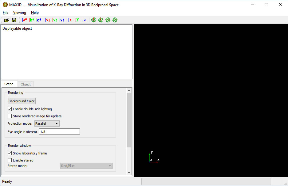
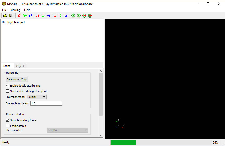
Double click on the MAX3D icon (which can be placed on the Desktop). The following GUI appears.
The right panel is the viewing area. The axes in the lower corner represent both the 3D volume space and the laboratory frame ( +X allong beam, +Z vertical, right handed )
The left panel lists the objects in the viewing area, and sets the scene and object visualization controls. The projection mode can be set to Perspective or Parallel. Mouse interaction can be set to Trackball ( simplest) or Joystick style.
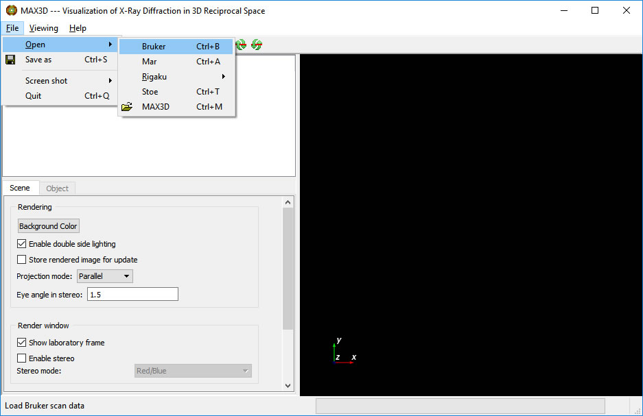
The File > Open pulldown offers several types of input. New readers are added as requested, time and funding permitting. The readers always need more testing . . .
Browse to a directory with, for this example, Bruker scans. At this point we are only selecting the folder.
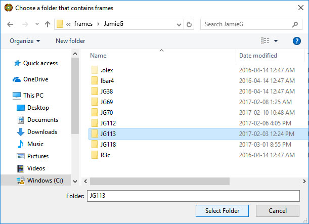
Choose the directory with a single click and press Select Folder.

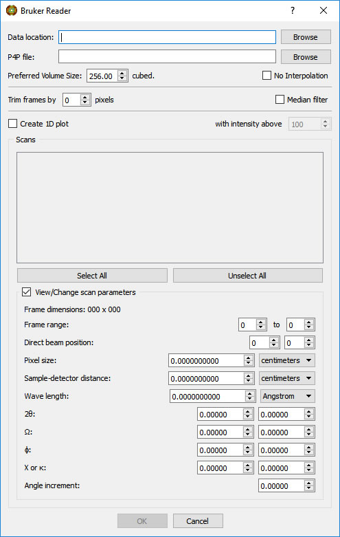
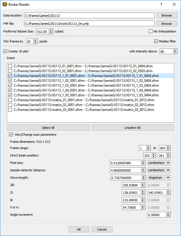
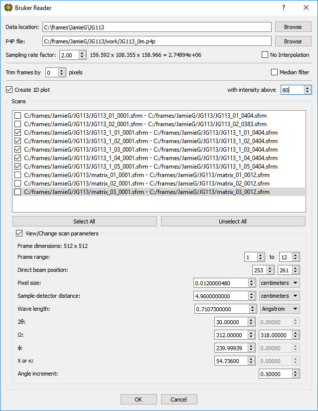
Select the appropriate scan(s). Information on the highlighted scan will be displayed. If you know that one or more parameters on the frame header are incorrect, you can insert the correct value(s). The corrections will be applied to all frames in the highlighted scan.
Options on the Reader menu include trimming pixels from the outer edge of the frames, median pixel smoothing to remove hot pixels, calculating a 1D Intensity (average or maximum) vs 2theta plot of the scan (useful for selecting 2theta ranges for pole figures - NOT a powder simulation unless the proper scans are done), and combining non-contiguous scans into one object without interpolation (useful for displaying residual stress data, for example).
Type in a preferred volume size. The number of voxels used will be the cube of this value. The volume loaded will have a rectangular shape to accommodate the scanned region od reciprocal space.
CAUTION: Be conservative to start. MAX3D does not poll the configuration of your computer, so asking for too large a volume can cause the program to hang. Later you will have the option to reload the data at higher resolution.
The examples shown here are from a 64bit Windows10 laptop with 16Gb RAM.
Browse for the Bruker .p4p file, if an orientation matrix has been previously determined.

Final scan selection and load parameters. Ready to go.
The progress of frame loading is displayed in the lower right corner. It usually starts fast and slows down. It should complete in a few minutes, depending on the requested resolution.
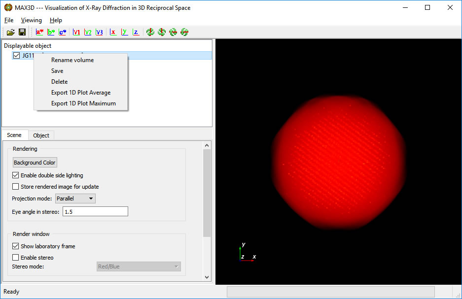
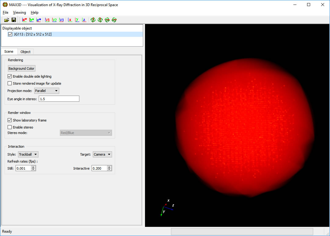
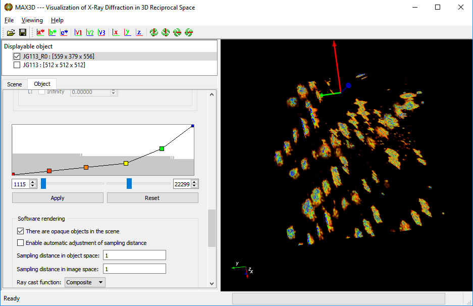
The complete volume will be displayed in the viewing area, and its name and size will be listed.
Once the volume is synthesized, you can righe click on the name and save an m3d file for later use. You have the option of renaming the volume. If 1D plots were requested, they can be saved.
The object can be rotated using the left mouse button, rotated around the viewing axis using ctrl-left button, panned using shift-left or center button, and zoomed using the right button.
If the software graphics control is used, the image will be at low resolution during motion.
The MAX3D window can be resized or made full-screen. the individual panels in the window can be readjusted, including filling the whole window with the image area.
Under the Scene tab there are options for setting the background colour, the projection mode (parallel or perspective), displaying lab axes, stereo settings, and mouse/mousepad interaction (trackball recommended).
Select the Object tab.
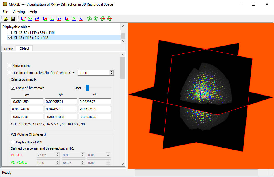
The outline of the selected volume can be toggled on or off, as can the reciprocal axes vectors.
In order to get better graphic response, make sure that the Graphics card option (GPU/GPU in Render Mode) is selected.
By default, the Viewing Style will be 3D View.
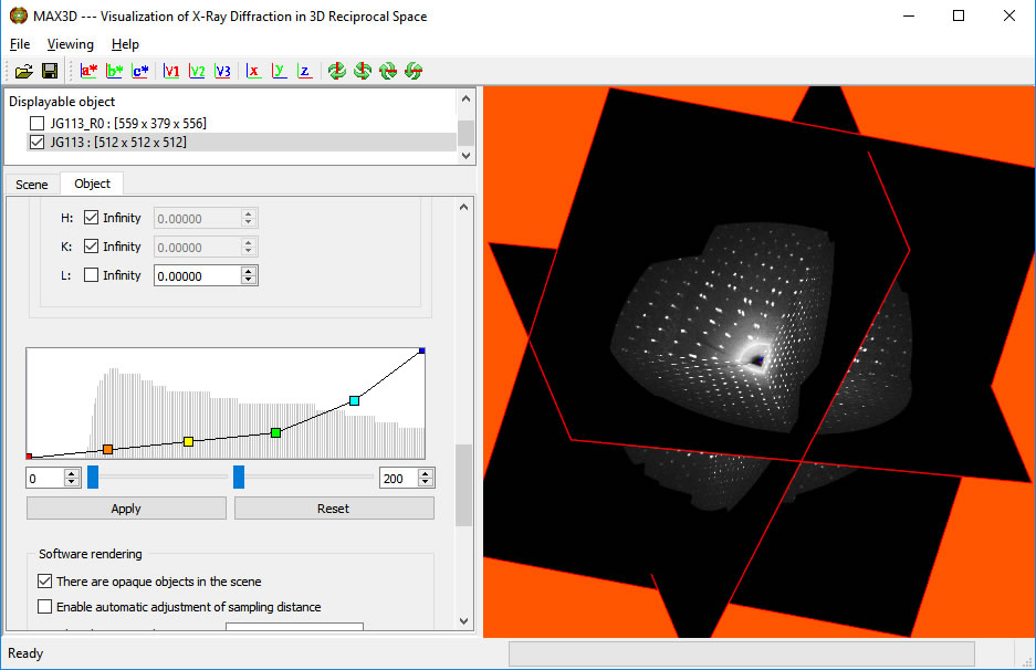
Scroll down to the plot of the 'transfer function'. The background histogram displays the populations (vertical) of increasing voxel intensity values (left to right). For most samples, the maxima represents the average frame noise level. The overlayed curve (straight line initially) controls the opacity of the voxels as a function of intensity. The intensity colour ramp is controlled by the coloured points on the transfer function curve.
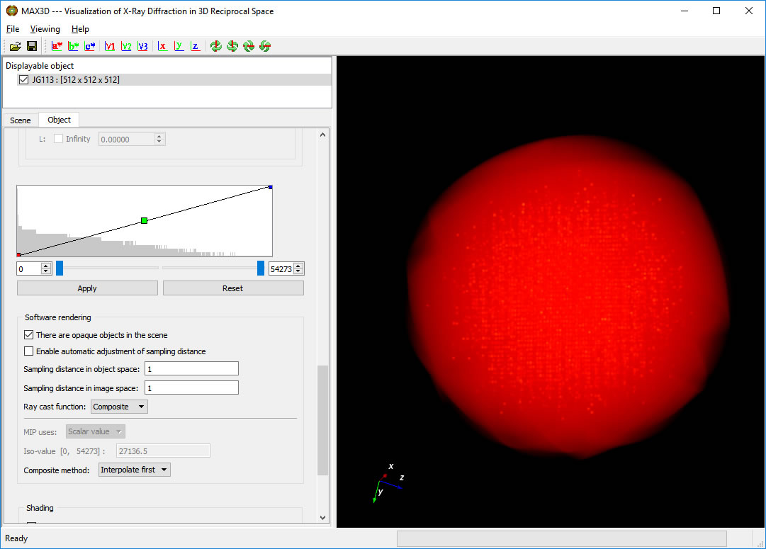
The lower and upper intensity limits (min and max voxel values) can be set to make the background scattering transparent and the more intense features constant.

Double clicking on a coloured point with the left button will bring up a choice of new colours for that point.
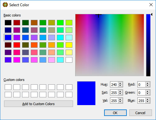
The coloured points on the transfer function curve are used as inflection points and can be moved with the left button to set the opacity levels as a function of intensity. New points can be added by placing the cursor on the curve and clicking the right button. Colours are interpolated automatically but can be reset. After a little practice, you can bring out the diffuse or weak features in your diffraction data. Zoom in for a closer look. At the moment, the displayed object is not at the full resolution of the collected data.

In order to get a more accurate look at the diffraction features of your sample, you need to select a subsection of the diffraction volume and reload the raw data with higher information density. Since the RAM of your computer limits the number of voxels which can be displayed at one time, it is necessary to work in a smaller volume of reciprocal space.
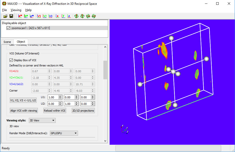
First, orient the object to a suitable viewing direction. You can use the view direction buttons on the upper toolbar. Then turn on the Volume of Interest (VOI) display box
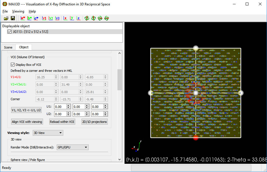
Click the 'Align VOI with viewing' button. You can then scale, rotate, reposition and reshape the VOI box using the handles and the faces. The box can can be sized uniformly with the right button. When using the handles to resize or reposition the box, the h,k,l position and 2theta value are displayed. When the cursor is over the box, the box is adjusted independently from the full object. The box will act as a 3D clipping volume. Moving the cursor outside of the box will allow you to zoom in and reorient the view. To view the isolated region of reciprocal space without the drawing of the box, simply uncheck the Display choice. The VOI box orientation vectors can be defined by identifying the principal U1 vector and a perpendicular U2 direction. Clicking the V1,V2,V3 button will orient the box. The V1, V2 and V3 buttons in the top icon bar can be used to set the viewing orientation. You can select any lattice volume, net or row you wish.
When the VOI is definedand the Box is displayed, click on the 'Reload within VOI' button. The Reader GUI will pop up, this time having a Scaling factor instead of a Volume size field.
Adjust the 'Sampling rate factor' to give a reasonable volume size.
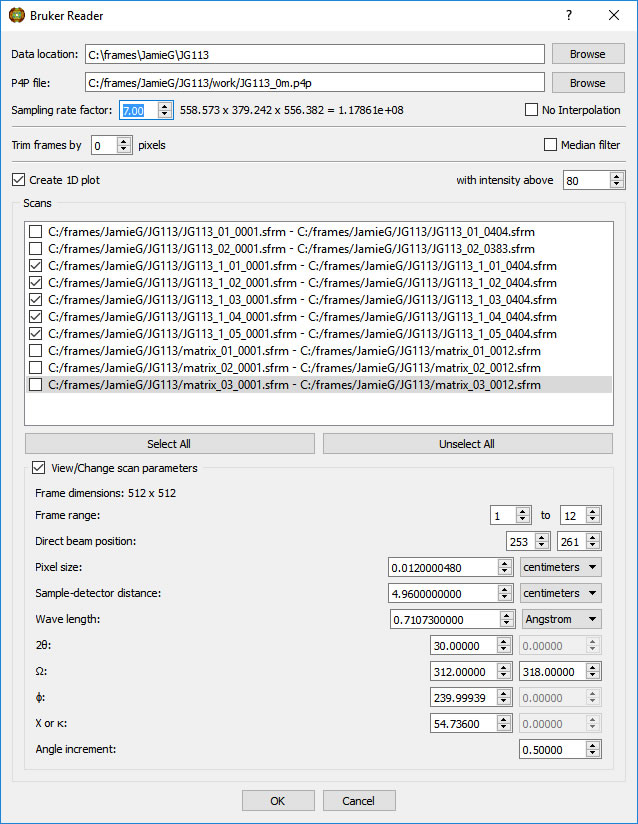
CAUTION: Do not ask for too high a voxel density. Your computer may complain (usually with work-to-rule tactics).
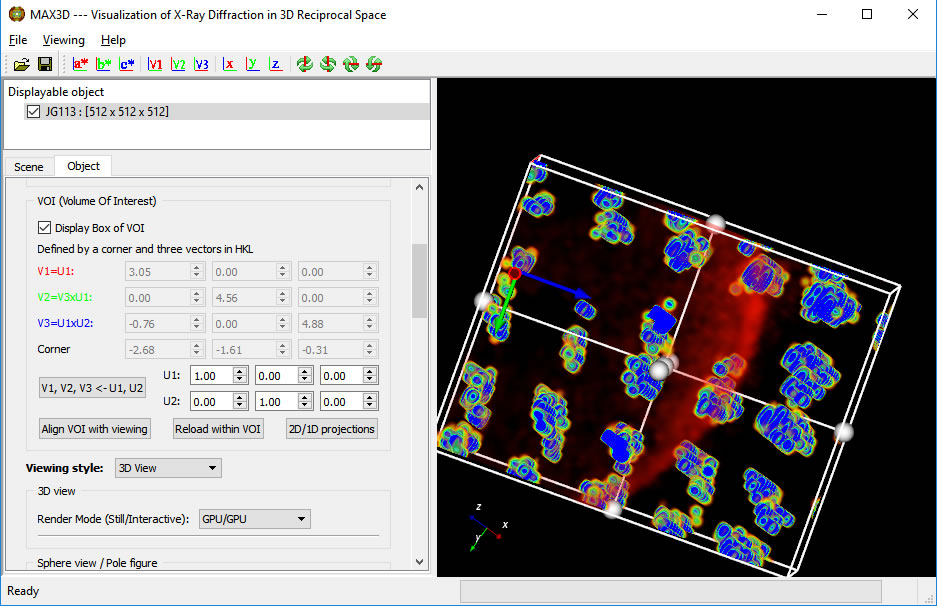
Click OK to start the reload. When it is complete, the new higher resolution object will be displayed in the same VOI. The original larger low resolution volume is still in memory and available to be viewed.
The transfer function can be set independently for the new volume.
A second Reload can give higher resolution images.
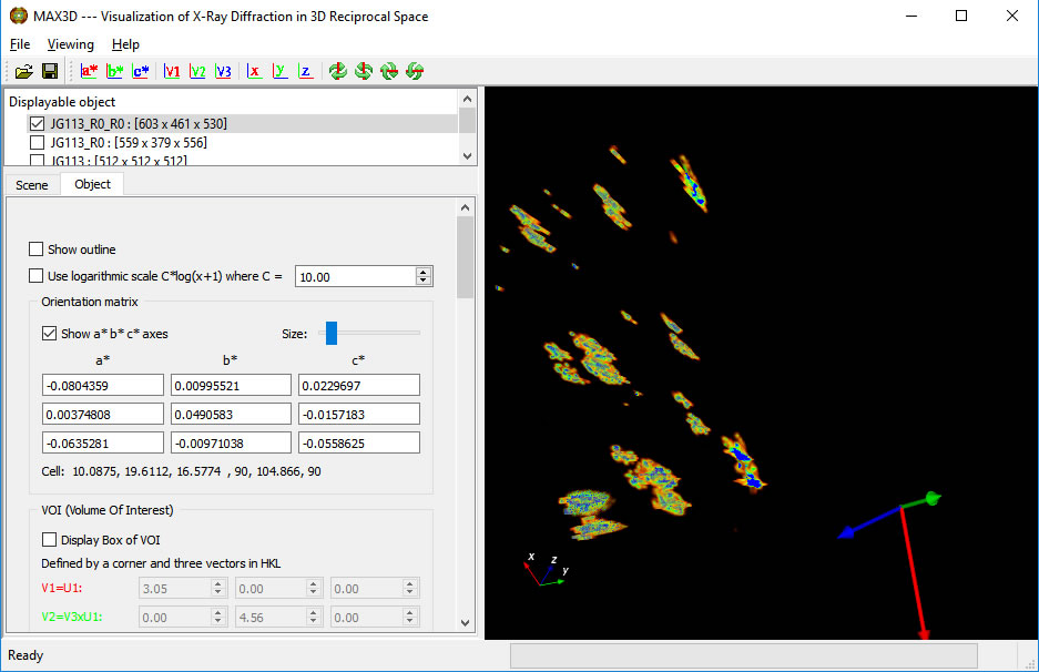
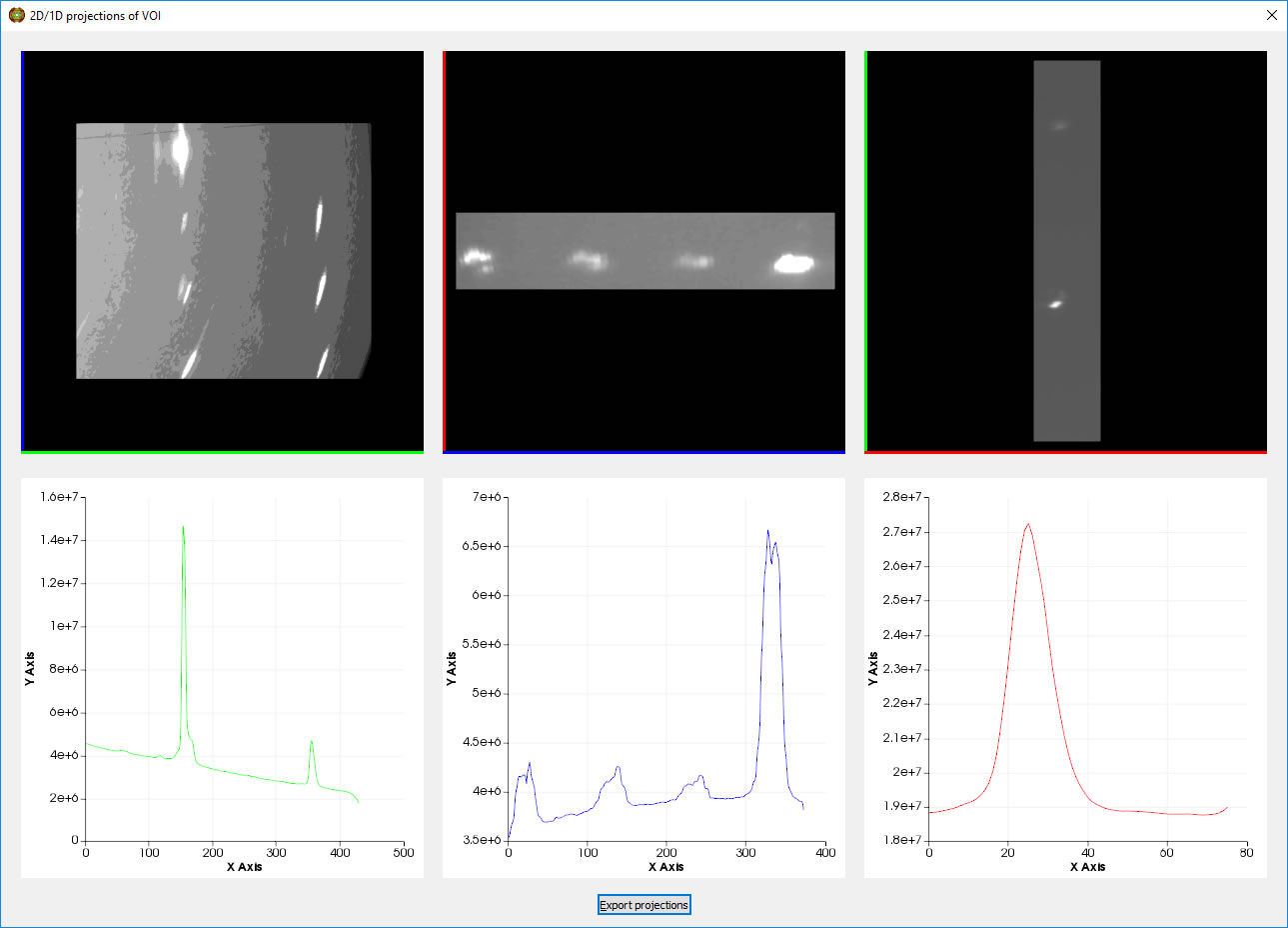
A new feature in V4.0 is the ability to select a specific orientation (using U1 and U2 fo define vectors V1, V2 and V3) of the volume in the VOI. Once the size of the VOI is set, you can calculate 2D and 1D projections.
The left mouse button can be used to adjust the brightness and contrast of the 2D windows. The projectins can be exported as csv files.
The Viewing style can be changed to Slice View. Reset the intensity range with the transfer function or the right mouse button. If you have loaded an orientation matrix, you can snap the slices to the reciprocal axes. The left mouse button can be used to identify positions and relative intensities. The planes can be moved or repositioned by typing positions into the slicing plane dialogue boxes or using the middle mouse button. Grabbing the face of a plane allows you to translate it along its normal direction. Grabbing the corner of a slice with a center click will allow rotation around its normal axis, while grabbing the edge allows rotation around the parallel in-plane axis.
You can use the MAX3D file loader to reload a a copy of the diffraction object and simultaniously display slices and 3D. By toggling the 3D image on and off, you can help navigate the slices through reciprocal space and identify features of interest.
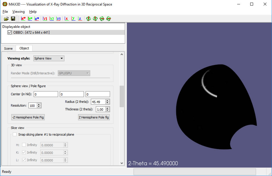
Once the brightness and contrast are setfor the slice view, you can explore reciprocal space with a 2q Sphere View. It can be dragged in and out using the right button with the cursor on the outer surface of the sphere. The 2q value will be displayed. (Great for picking out pole figures in texture data.) A left button click on the surface displays the hkl values of the point. The view can be changed with the cursor away from the surface. The mouse wheel or right edge of the mouse pad can be used for scaling.

The Sphere resolution can be increased to improve the image. This will, however, reduce the graphical response time.
CAUTION: Step up in jumps of 100 and test the response. Overtaxing your graphics driver can result in
the blue screen of death!
As well as m3d files and 2D and 1D projections, snapshots of the viewing area can be saved.

You can record an mpeg video from the Scene tab by selecting a file location (include the .mpg extension) and Start. Recording will only take place while the object is being moved. You can also record a screen-dumped avi video or streaming video using a program such as CamStudio. The latest version of Microsoft Office PowerPoint has a nice screen video capture function. Examples of videos will be available form the main MAX3D website (http://max3d.mcmaster.ca/).
A new feature of MAX3D is the ability to examine XRD3 texture (grain orientation) data and generate 3D thick shells for view pole figures.
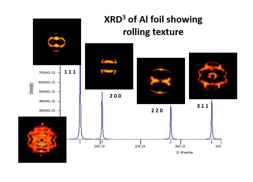
Below is a 120 degree collection of XRD3 data from a fibre-textured film on a substrate (Oakley, Lekin, University of Waterloo) using Co radiation and a Bruker Vantec500 detector.
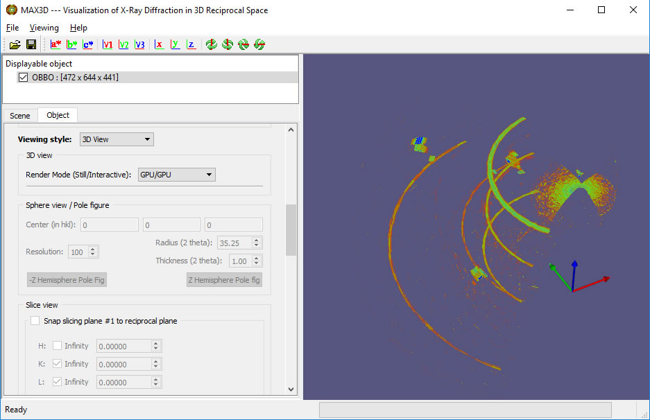
Sphere view can be used to identify a the 2Theta value of a select diffraction feature.
The View can be switched to Pole Figure and the thickness of the shell can be adjusted.
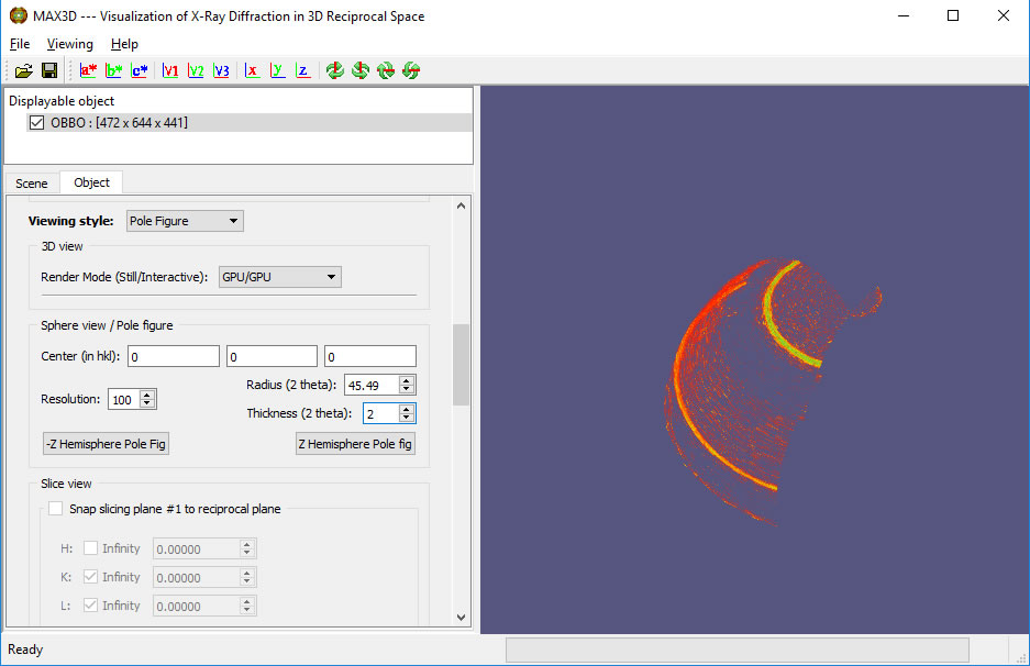
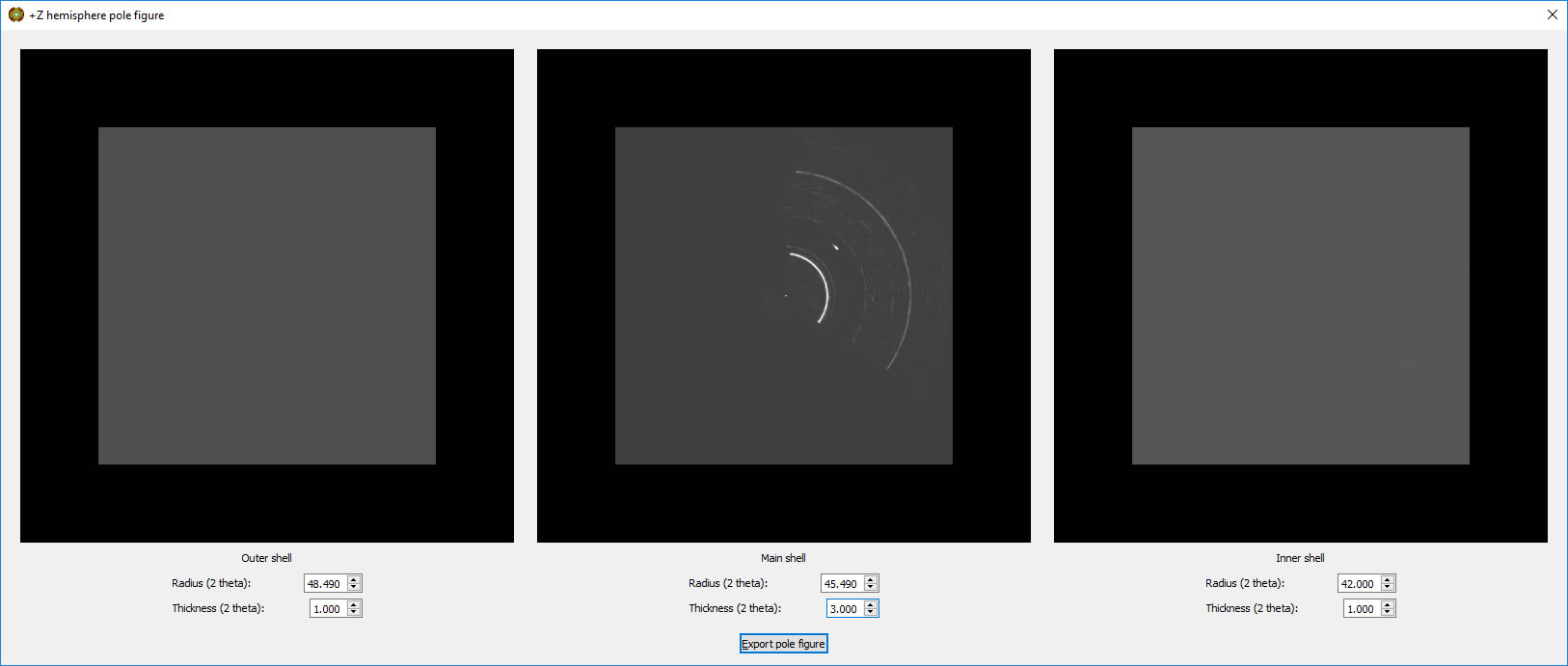
The Z Hemisphere Pole fig button allows you to generate a stereographic projection of the shell, tune its thickness and adjust the background subtraction regions above and below the shell. A Bruker style .gpol frame of the background corrected pole figure can be exported, suitable for input to the MTex texture analysis module in MatLab.
MAX3D has been supported by a series of SharcNet Dedicated Programming awards. Thanks go to Ranil Sonnadara for making this happen. We would also like to acknowledge Mark Hollingsworth of Kansas State University and Joe Ferrara of Rigaku Americas Corporation for development support.
MAX3D will be under slow but steady development as will this User Manual. Bug fixes, new readers, new tools, and new ideas will be incorporated. Your input, as well as links to interesting results, will be greatly appreciated. Have fun exploring!